A* vs RRT Path Planning Explained (September 2026)

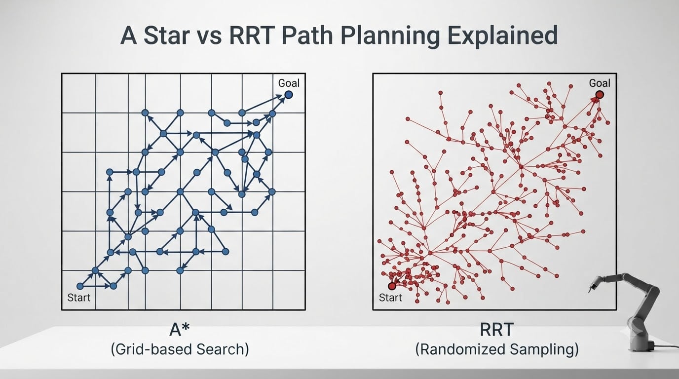
If you’ve ever wondered how a robot decides where to move, you’ve landed in the right place. Path planning is the brain behind every autonomous system, and two algorithms dominate the conversation: A* (A-Star) and RRT (Rapidly-exploring Random Tree). I work with both regularly in robotics projects, and each one has clear strengths, clear weaknesses, and a clear set of use cases where it shines.

In this guide, I’ll break down exactly how A* vs RRT path planning works, where each algorithm wins, and how to choose the right one for your project. Whether you’re programming a mobile robot, a 7-DOF robotic arm, or a simulated agent in a game, this comparison will give you a decision framework you can actually use.

By the end, you’ll understand the math behind both algorithms, see a side-by-side comparison table, and know which one to reach for in high-dimensional spaces, real-time systems, and grid-based environments. If you’re also working through related robotics fundamentals, our breakdown of forward kinematics vs inverse kinematics pairs well with the manipulator examples below.

What is A* Path Planning Algorithm

A* is a graph search algorithm that finds the shortest path between a start node and a goal node using a heuristic to guide its exploration. It was first described in 1968 by Peter Hart, Nils Nilsson, and Bertram Raphael, and it remains the workhorse for grid-based path planning in robotics and games.

The core idea is elegant: A* evaluates each candidate node using the formula f(n) = g(n) + h(n), where g(n) is the actual cost from the start to node n, and h(n) is a heuristic estimate of the cost from n to the goal. The algorithm always expands the node with the lowest f-score next, which gives it a powerful balance between following what it knows (g) and predicting what it needs (h).

This makes A* both complete (it will find a path if one exists) and optimal (it will find the cheapest path) as long as the heuristic is admissible, meaning it never overestimates the true cost. Common admissible heuristics include Manhattan distance for 4-connected grids and Euclidean distance for continuous spaces.

How A* Works Step by Step

I’ve implemented A* from scratch multiple times, and the algorithm flow is consistent across languages. Here is the step-by-step process:

Step 1: Initialize two lists. The open set holds nodes to be evaluated (often a priority queue sorted by f-score), and the closed set holds nodes already evaluated. Add the start node to the open set with g(start) = 0.

Step 2: Pop the node with the lowest f-score from the open set. If it’s the goal, reconstruct the path by following parent pointers backward and return.

Step 3: Move the current node to the closed set. For each neighbor, calculate a tentative g-score. If the neighbor is in the closed set and the new g is higher, skip it.

Step 4: If the neighbor is not in the open set, or the new g-score is lower than its existing g, update its g and f scores, set its parent to the current node, and add it to the open set.

Step 5: Repeat from Step 2 until the goal is found or the open set is empty (meaning no path exists).

Heuristic Function Deep Dive

The heuristic is what separates a fast A* from a painfully slow one. A perfect heuristic would guide A* directly to the goal with zero wasted exploration, but perfect heuristics are usually impossible to compute without solving the problem itself.

For a 2D grid, Manhattan distance |dx| + |dy| works well for 4-directional movement. For 8-directional movement, the octile distance (scaled Manhattan for diagonals) is better. For continuous spaces, Euclidean distance is the standard pick. The key constraint is admissibility: the heuristic must never overestimate, or A* loses its optimality guarantee.

Strengths and Limitations of A*

A* is fast on grid maps, returns optimal paths when given an admissible heuristic, and is straightforward to implement. It powers pathfinding in everything from Warcraft III to modern warehouse robots.

The big limitation is the curse of dimensionality. A* expands nodes in the configuration space, and that space grows exponentially as you add dimensions. A 6-DOF robotic arm has a configuration space that is essentially impossible to discretize finely enough for A* to be practical. That’s where RRT enters the picture.

What is RRT Path Planning Algorithm

RRT (Rapidly-exploring Random Tree) is a sampling-based path planning algorithm designed by Steven LaValle in 1998. Instead of systematically searching a grid, RRT builds a tree of collision-free states by randomly sampling the configuration space and connecting each new sample to the nearest existing node.

The result is a tree that rapidly explores the reachable space, with branches that grow toward unexplored regions. RRT is probabilistically complete: as the number of samples approaches infinity, the probability of finding a path (if one exists) approaches 1. However, the path it returns is not guaranteed to be optimal.

How RRT Works Step by Step

RRT is refreshingly simple compared to A*. The core algorithm is short enough to fit in a single function. Here is the step-by-step breakdown:

Step 1: Initialize the tree with the start configuration as the root node.

Step 2: Generate a random sample in the configuration space. Most implementations use a small probability (around 5 to 10 percent) of sampling the goal directly, which biases the tree toward the goal without sacrificing exploration.

Step 3: Find the node in the tree nearest to the random sample. This is typically done with a KD-tree for performance, especially in high-dimensional spaces.

Step 4: Extend from the nearest node toward the random sample by a fixed step size. If the resulting new node is collision-free, add it to the tree as a child of the nearest node.

Step 5: Check if the new node is within a goal tolerance of the goal configuration. If so, return the path by tracing parent pointers from goal to start.

Step 6: Repeat from Step 2 until a path is found or the iteration limit is reached.

Why Sampling Works in High Dimensions

The reason RRT dominates high-dimensional planning comes down to probability. In a 2D grid with 100 by 100 cells, A* might need to evaluate 10,000 nodes. In a 6-DOF arm, the equivalent configuration space is 10 to the 12th power nodes, which is computationally infeasible.

RRT sidesteps this by never explicitly representing the free space. It only checks collision along a line segment between the nearest node and the new sample, and it does this O(n) times where n is the number of samples. As long as the underlying collision checker is fast, RRT scales gracefully to 7, 10, or even 20 degrees of freedom. This is why RRT and its variants are the default choice in MoveIt, OMPL, and most modern robotic manipulation stacks.

RRT Variants: RRT* and Informed RRT*

RRT returns the first path it finds, which is usually suboptimal. RRT* fixes this by adding a rewiring step: after adding a new node, RRT* checks nearby nodes (within a ball of shrinking radius) and rewires the tree if a cheaper parent exists. RRT* is asymptotically optimal, meaning the path cost converges to the optimum as the number of samples goes to infinity.

Informed RRT* takes this further. Once a first solution is found, Informed RRT* restricts all subsequent sampling to the heuristic-informed ellipsoid that contains all configurations that could improve the current best path. This dramatically speeds up convergence to near-optimal solutions in practice, and it is the variant I reach for most often when planning for robotic arms.

A* vs RRT Comparison Table

Here is the side-by-side comparison I wish I had when I first started working with both algorithms. The table below covers the dimensions that matter most for engineering decisions.

Search approach: A* uses systematic graph search with a heuristic. RRT uses random sampling in the configuration space.

Optimality: A* is optimal with an admissible heuristic. RRT is not optimal by default, but RRT* is asymptotically optimal.

Completeness: A* is complete on finite graphs. RRT is probabilistically complete.

Best dimensionality: A* works best in 2D and 3D grids, generally up to 4 or 5 dimensions. RRT scales well to 7+ DOF configurations.

Path quality: A* returns the shortest path on the discretized grid. RRT returns a feasible but typically longer path.

Memory usage: A* stores all visited nodes, growing with grid size. RRT only stores the tree, growing with the number of samples.

Typical use cases: A* fits game AI, warehouse navigation, and grid maps. RRT fits robotic arms, drone planning, and high-DOF manipulators.

Implementation complexity: A* is moderate, around 100 lines of code. RRT is simpler at the core, but needs a good collision checker and nearest-neighbor structure.

Real-time performance: A* is deterministic and predictable. RRT runtimes vary by seed, which can complicate real-time guarantees.

RRT vs RRT* Key Differences

RRT and RRT* look almost identical in code, but their behavior diverges sharply once you care about path quality. The core difference is the rewiring step in RRT*.

In RRT, when you add a new node x_new, you connect it to the single nearest neighbor. That connection is final. In RRT*, after connecting x_new to its nearest neighbor, you search all nodes within a radius r of x_new. For each of those nearby nodes, you check whether going through x_new would produce a cheaper path from the start. If so, you rewire the tree: x_new becomes the new parent of that node.

The radius r shrinks as the number of nodes grows, following the formula r = gamma times (log n divided by n) to the power of 1 divided by d, where d is the dimensionality. This shrinking radius is what gives RRT* its asymptotic optimality guarantee. In practice, RRT* often takes 5 to 10 times longer than RRT to find a first solution, but the path quality is significantly better, and it keeps improving with more iterations.

Informed RRT* extends this further by sampling only inside the heuristic-informed ellipsoid after a first solution is found. If you’re planning for a robot arm where the initial RRT path zigzags through free space, Informed RRT* is usually the better default in 2026.

Algorithm Complexity Analysis

Computational complexity is where A* and RRT diverge most clearly. A* has a time complexity of O(b^d) in the worst case, where b is the branching factor and d is the depth of the solution. With a perfect heuristic, this drops to O(d). Memory is O(b^d) because A* must store all expanded nodes in the worst case.

RRT has a more nuanced complexity story. Each iteration requires a nearest-neighbor query and a collision check along the new edge. With a KD-tree, the nearest-neighbor query is O(log n). The collision check depends on the environment, but for a robotic arm checking a 7-DOF configuration, each check is typically a few milliseconds.

In practice, this means A* is faster than RRT for small grid maps but becomes completely impractical for high-dimensional configuration spaces. A researcher in a Reddit thread I read put it well: A* outperforms RRT in 3D scenarios for both path length and computational time, but the moment you go beyond 4 or 5 dimensions, the comparison flips.

For real-time applications, A* is generally more predictable because its runtime depends on the graph size, not on random sampling. RRT runtimes can vary by 30 to 50 percent between runs with different seeds, which complicates worst-case timing guarantees.

High-Dimensional Space Handling

High-dimensional configuration spaces are where RRT and its variants earn their keep. A 7-DOF robotic arm has a 7-dimensional configuration space, where each dimension corresponds to a joint angle. A* would need to discretize this space finely enough to find valid paths, which means millions or billions of nodes.

RRT avoids this by sampling. The probability of a random sample landing in a valid region of free space is roughly the volume of free space divided by the total volume. Even in 7D, if the free space is reasonably large, random sampling will find a path with a few thousand samples.

This is why MoveIt, the most widely used motion planning framework for ROS, uses OMPL (Open Motion Planning Library) under the hood, and OMPL defaults to RRT-Connect and RRT* for manipulation tasks. When you’re working with a Franka Panda arm or a UR5, RRT-family algorithms are doing the planning work.

For mobile bases in 2D environments, the calculus flips. A* on a 2D occupancy grid is fast, deterministic, and gives you optimal paths. That’s why autonomous vehicles in structured environments often use A* or its successor, Hybrid A*, which adds kinematic constraints like vehicle turning radius.

When to Use Each Algorithm

Here’s the decision framework I use when choosing between A* and RRT for a new project. It comes down to four questions:

Question 1: How many dimensions? If your configuration space is 2D, 3D, or low-dimensional, start with A*. If it’s 4D or higher, RRT-family algorithms are almost always the better choice.

Question 2: Do you need the shortest path? A* returns the optimal path on a discretized grid. If you need the absolute shortest path and your space is grid-friendly, A* wins. If you need a feasible, near-optimal path, RRT* or Informed RRT* is the right pick.

Question 3: Is your environment dynamic? A* requires a full re-search when the environment changes. RRT-based incremental planners like RRT# or dynamic RRT can reuse the existing tree, which is much faster in dynamic environments.

Question 4: Is real-time determinism critical? A* has predictable runtime based on graph size. RRT runtime varies by seed. For hard real-time systems where worst-case latency matters, A* (or precomputed A* variants) is safer.

For game AI, A* is almost always the right answer. For warehouse robots, it depends on the warehouse size. For autonomous vehicles, Hybrid A* handles the kinematic constraints better. For robotic arms, RRT* is the industry default.

Implementation Considerations

When you’re ready to implement these algorithms, here are the practical considerations I’ve learned the hard way. First, don’t reinvent the wheel unless you need to. OMPL, MoveIt, and the Python Robotics library all have tested, optimized implementations of A*, RRT, and RRT*.

If you’re implementing A* yourself, the priority queue is the most important data structure. Python’s heapq works, but for larger grids, a binary heap with proper decrease-key handling is faster. Always use a consistent heuristic, and always check that the heuristic is admissible before claiming optimality.

For RRT, the collision checker is the bottleneck. Invest time in a fast, vectorized collision check. For a 7-DOF arm, libraries like FCL (Flexible Collision Library) and PyBullet can speed up collision checks by 10x compared to naive implementations.

Parameter tuning matters more than people expect. For RRT, the step size should be roughly 1 to 5 percent of the configuration space diameter. Too small, and you waste samples on tiny branches. Too large, and you miss narrow passages. Goal biasing at 5 to 10 percent usually improves convergence without hurting exploration.

If you’re comparing microcontrollers for running these algorithms, our comparison of Arduino vs Raspberry Pi vs ESP32 covers the hardware side. Spoiler: A* on a grid runs fine on an ESP32, but RRT for a 6-DOF arm needs a Raspberry Pi 4 or better.

Real-World Applications

A* and RRT show up in very different industries because they’re solving different problems at their core. Game AI is the classic A* domain. Pac-Man, StarCraft, and Diablo all use A* (or variations like IDA* and JPS) for unit pathfinding. The grid is small, the heuristic is obvious, and optimality matters for predictable AI behavior.

Warehouse robots from Amazon and Kiva Systems use A*-style planners on 2D occupancy grids. The robots move in structured environments with clear corridors, and optimal path length translates directly to faster order fulfillment. The same approach shows up in drone delivery planning for low-altitude urban navigation, where 2D or 2.5D grid planners are the norm.

Robotic arm manipulation is RRT territory. Industrial arms from ABB, KUKA, and Fanuc all use RRT* variants internally for collision-free motion planning. The configuration space is high-dimensional, obstacles are complex, and near-optimal paths are good enough as long as the motion is smooth.

Autonomous vehicles blend both worlds. Behavior planning often uses search-based methods like Hybrid A* for lane-level path planning, while motion planning in parking and complex maneuvers uses RRT* or optimization-based planners. Recent industry moves like the partnership covered in HII’s $900M agreement with Path Robotics and GrayMatter Robotics show that hybrid approaches combining graph search and sampling are where the industry is heading.

One more emerging area is the 3.3V vs 5V logic choice in embedded robotics hardware, which we covered in our 3.3V vs 5V guide. Choosing the right logic level matters when your path planner is running on an embedded board.

Frequently Asked Questions

Conclusion

A* vs RRT path planning is not really a competition. They are tools for different jobs, and choosing the right one depends on your configuration space, optimality requirements, and runtime constraints.

Use A* when you’re working in 2D or 3D grids and you need the shortest path with predictable runtime. Use RRT when your robot has 4 or more degrees of freedom and the configuration space is too large to discretize. Use RRT* or Informed RRT* when you need near-optimal paths in high-dimensional spaces.

For most robotics projects in 2026, start with the simplest algorithm that solves your problem. Profile it, identify the bottleneck, and only then reach for a more sophisticated planner. Our team has used this approach to ship manipulation stacks, mobile robots, and autonomous systems without over-engineering the planning layer.