Why My Simulated Robot Behaves Differently in Real Life (September 2026)

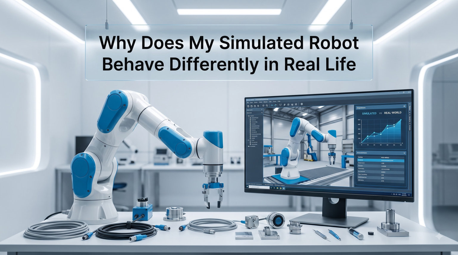
You spend three days training a quadruped in simulation. Reward curves look great, the robot walks smoothly, and your video clip is ready to post. Then you flash the policy to the real hardware, and the robot immediately falls over, twitches, or wanders into a wall.

If that scene feels familiar, you have hit the sim-to-real gap. It is the single most common reason a simulated robot behaves differently in real life, and it is the reason almost every serious robotics team in 2026 still budgets time and money for physical testing. In this guide, I will walk you through what the gap is, why it exists, and the specific techniques our team uses to shrink it.

You will learn the four core causes of the gap, the difference between domain randomization and system identification, when each one works, and a practical diagnostic checklist for figuring out exactly which assumption your simulation is making incorrectly. By the end, you will have a clear plan for turning a sim-trained policy into one that survives first contact with the real world.

What Is the Sim-to-Real Gap in Robotics?

The sim-to-real gap is the performance drop that happens when a robot policy trained in simulation is deployed on physical hardware. A policy that achieves 95% success in simulation can drop to 20% on a real robot, even when the code is identical. That difference is the gap.

Think of simulation as a sketch and the real world as the finished painting. Both depict the same scene, but the sketch uses simple lines while the painting has texture, light, and small imperfections. The sim-to-real gap is the space between the sketch and the painting.

Robotics teams care about this gap because simulation is fast, cheap, and safe. You can train millions of episodes overnight without wearing out motors or risking injury. The promise of sim-to-real transfer is that you get all of that benefit and still end up with a working real-world policy. Closing the gap is what makes that promise real.

The four main sources of the gap are:

• Physics approximations in the simulator, especially contact and friction models.
• Sensor noise and bias that simulators usually model too cleanly.
• Actuator dynamics that differ between ideal motors and real gearboxes, servos, and current loops.
• Environment mismatch in lighting, surface properties, and object masses that never quite match the lab.

If you have asked yourself why does my simulated robot behave differently in real life, the answer is almost always a combination of those four factors, not just one. The rest of this guide shows you how to identify which ones are biting you.

Why Simulation Differs from Reality: Core Causes of the Gap

Every physics simulator is a tradeoff between speed and accuracy. A simulator that ran at the fidelity of molecular dynamics would never finish an episode, so engineers make simplifying assumptions. Those assumptions are where the gap starts.

1. Physics Approximations in the Simulator

Most popular simulators (MuJoCo, PyBullet, Isaac Sim, Genesis, Bullet) use rigid body dynamics with simplified contact solvers. That means objects do not deform, do not have thermal properties, and bounce off each other using penalty or constraint methods that approximate but do not exactly replicate real collisions.

Friction is especially tricky. Real friction depends on surface finish, temperature, dust, humidity, and contact area. A simulator usually gives you a single friction coefficient per pair of materials. When you set friction in code, you are not capturing reality; you are picking one number that represents a wide range of conditions.

2. Sensor Noise and Bias

In simulation, an IMU is usually modeled as a clean signal plus Gaussian noise. In reality, IMUs drift with temperature, exhibit bias instability, and saturate during high-acceleration events. Cameras have rolling shutter, motion blur, depth-of-field, and lens distortion. LiDAR returns have multi-path artifacts. If your simulation does not model these, your policy is learning on a cleaner stream of data than it will see in the real world.

3. Actuator Dynamics

Simulated motors usually respond to torque commands instantly and proportionally. Real motors have current limits, thermal limits, backlash, friction in the gearbox, and PWM frequency effects. A policy that commands a torque spike that the real motor cannot deliver will look fine in sim and break on hardware. If you are also seeing motor driver overheating problems on the real robot, the actuator model is a strong suspect.

4. Environment Mismatch

Even if your robot is perfectly modeled, the world around it is not. Table surfaces flex, floors are not perfectly flat, objects weigh a few grams more or less than the spec sheet claims, and lighting changes throughout the day. A policy that memorizes visual features in the simulator will fail when those features shift. We cover a related symptom in our guide on robot chassis design, where small mechanical differences cascade into large behavioral changes.

How Physics Engines Approximate the Real World

To fix the gap, it helps to understand how a simulator actually steps forward in time. Most simulators use fixed-step numerical integration, usually at 1 kHz or higher, with a smaller inner loop for contact resolution. The integrator takes the current state, computes forces, and updates velocities and positions using something like semi-implicit Euler or a Runge-Kutta method.

That math is accurate when forces change slowly, but it can drift when forces are stiff or discontinuous, which is exactly what happens during contact. To handle contacts, simulators add a separate solver that tries to keep objects from interpenetrating while respecting friction cones. Common approaches include penalty methods, LCP (linear complementarity problem) solvers, and impulse-based methods.

Each method has tradeoffs. Penalty methods are fast but allow some interpenetration. LCP solvers are more accurate but slower and can fail on stiff contact stacks. Impulse methods handle impacts well but struggle with sustained contact. None of them is the real world. They are each a useful approximation, and the gap is the difference between that approximation and the messy physical world you care about.

This is also why tuning timestep matters. If your simulator runs at 1 ms but your real controller runs at 10 ms, your policy is being trained on a different effective control frequency. That alone can cause a real robot to behave differently from the simulated robot.

Domain Randomization: The Brute-Force Approach

Domain randomization is the most common practical solution to the sim-to-real gap. Instead of trying to make the simulator perfectly accurate, you randomize the simulator. During training, you vary physics parameters, sensor noise, lighting, and object properties across a wide range. The policy then learns to be robust to all of them, including the version that happens to match reality.

The insight is simple: if your policy works across a wide enough distribution of simulated worlds, it will probably work on the real one, because the real world is just one more sample from that distribution.

What to Randomize First

If you are starting from scratch, the parameters with the highest payoff are usually:

• Mass and inertia of the robot’s links and any objects it interacts with. A 10% mass error can change manipulation behavior dramatically.
• Friction coefficients between gripper and object, and between wheels or feet and the ground.
• Motor strength and response delay, including current limits and a small amount of random latency.
• Sensor noise, especially IMU bias and camera brightness or contrast shifts.
• Visual appearance for vision-based policies, including lighting direction, color jitter, and texture randomization.

Start with conservative ranges (for example, plus or minus 20% on mass) and expand them only if real-world tests show you are still overfitting to simulation.

A Minimal Example

Here is a simplified Python snippet that shows the idea. It uses a generic gym-style environment API, so the structure transfers to most simulators.

import random

def randomize_env(env):
    # Vary mass of the target object
    env.object.set_mass(random.uniform(0.8, 1.2))

    # Vary friction between gripper and object
    env.gripper.set_friction(random.uniform(0.5, 1.5))

    # Add a small random delay to actuator response
    env.actuator.set_delay(random.uniform(0, 0.02))  # seconds

    # Randomize lighting for vision-based policies
    env.camera.set_brightness(random.uniform(0.7, 1.3))
    env.camera.set_noise_stddev(random.uniform(0.0, 0.05))

The downside of domain randomization is training time. If your randomization range is too wide, the policy may never converge. If it is too narrow, it will overfit and fail on the real robot. Tuning these ranges is a skill in itself, which is one reason we recommend a hybrid approach later in this guide.

System Identification: The Precise Approach

System identification is the opposite philosophy. Instead of randomizing, you measure the real robot carefully and feed those measurements back into the simulator. The goal is to make the simulator match the real robot as closely as possible, then train a policy in that high-fidelity simulator with little or no randomization.

Common measurements include:

• Link masses and centers of mass, measured by hanging each part and locating the balance point.
• Motor constants, including torque per amp and back-EMF, from a brief bench test.
• Friction coefficients, measured by dragging a part across the actual surface with a force gauge.
• Sensor noise profiles, recorded by leaving the sensor still for a few minutes to capture bias and drift.

System identification works best for robots with few degrees of freedom and tasks that are sensitive to small parameter errors, like precision manipulation. It works less well for legged locomotion, where the parameter space is huge and the simulator needs to be right about dozens of things at once.

Limitations

No measurement is perfect. Your friction measurement is for one specific surface, one specific day, one specific dust level. Even with great system identification, the real robot will still behave slightly differently from the simulated robot. That is why most teams use system identification as a starting point and then layer domain randomization on top.

Hybrid Methods: Combining Randomization and Identification

In our team’s experience, the most reliable results come from a hybrid approach. We use system identification to set the baseline parameters, then randomize within a small range around those values during training. The narrow range keeps training fast while still giving the policy some robustness to the residual gap.

Other hybrid techniques have become popular in 2026:

• Teacher-student training, where a teacher policy trained in sim is distilled into a student policy that only sees real sensor inputs.
• Fine-tuning on small amounts of real-world data after sim training.
• Privileged information, where the teacher gets clean sim state and the student learns to recover that state from noisy real sensors.
• Adaptive domain randomization, where the training distribution is automatically widened or narrowed based on the policy’s behavior.

Each of these is an answer to the same question: how do I get a policy that does not need a perfect simulator but still works on imperfect hardware? You will notice that this is exactly the failure mode of policies that ignore the issue, where a robot browning out and resetting under load is treated as a power problem when it is really an actuator model problem.

Troubleshooting: Diagnosing Why Your Simulated Robot Behaves Differently

This is the section most guides skip, and it is usually the section you actually need. When a policy fails on the real robot, the first job is figuring out which assumption is wrong. Here is a diagnostic checklist our team runs through, roughly in order of likelihood.

Step 1: Check the Control Frequency

Confirm that the simulated policy and the real policy are running at the same loop rate. A mismatch of even 5 ms can change a policy’s behavior. If your real controller is slower than sim, that alone can cause the robot to fall over or oscillate. Fix this first because it is the easiest to verify.

Step 2: Inspect the Actuator Model

Send a step torque command to the real motor and log its response. If the response is much slower or faster than your simulator predicts, your actuator model is wrong. Increase the simulated motor response time, or add a saturation block. If you are also seeing Raspberry Pi crashing under compute load when the policy runs, your actuator delay is likely being amplified by missed deadlines.

Step 3: Test on a Single Joint

Lock everything except one joint and run the policy on that joint only. If the joint tracks well, the issue is likely multi-joint dynamics or contact. If the joint fails, the issue is in your low-level actuator or sensor stack. This isolates the problem in minutes.

Step 4: Log Real Sensor Data and Replay It in Sim

Record a real rollout and feed the exact same sensor stream into your simulator. If the policy now succeeds in sim with the real data, the gap is in your sensor model. If it still fails, the gap is in the dynamics. This trick is the single fastest way we have found to localize the problem.

Step 5: Compare Contact Behavior

Place the real robot in a controlled contact task, like pressing against a force gauge, and compare the measured forces to what the simulator predicts. Big mismatches here point to a friction or contact stiffness problem. Small mismatches across many contacts point to mass or inertia errors.

Step 6: Visualize the Failure

Record video of the real failure and the sim rollout side by side. Even when the sim and real look similar at the start, the divergence usually happens at a specific moment. That moment is your cue. It might be the first contact, the first rapid direction change, or the first time the robot approaches an object. Zoom in on that frame and check the simulator’s prediction.

Step 7: Widen Randomization, Then Narrow It

If the failure is in dynamics, double the randomization range, retrain for a short time, and test again. If performance improves, the gap is being closed by the wider distribution. If it gets worse, your randomization is now too aggressive and the policy is failing to learn. Narrow the range and try again. This loop is the most reliable way to find the right randomization width for your specific robot.

One more practical note: when you are chasing a stubborn sim-to-real bug, the failure is rarely the one thing you most recently changed. Walk back through your last few commits and look for the parameter that moved the simulation further from reality. That is almost always where the gap widened.

Frequently Asked Questions

Closing Thoughts on Closing the Sim-to-Real Gap

The sim-to-real gap is not a bug. It is a property of the fact that simulations are models and the real world is not. Every robotics team in 2026 faces it, and the teams that ship reliable robots are the ones that budget for it explicitly rather than hoping it will not show up.

Start by understanding which assumption is breaking: physics, sensors, actuators, or environment. Use system identification to set a baseline, then randomize within a narrow range around those values. Run the diagnostic checklist the moment a real-world rollout fails, and treat the first failure as data, not as a setback.

If you keep one thing from this guide, keep this: the question is not whether your simulated robot will behave differently in real life, but how quickly you can find out which assumption is wrong and fix it. That is the work of robotics, and the teams that do it well are the ones that build policies that survive first contact with the real world.