Forward Kinematics vs Inverse Kinematics Explained (2026)

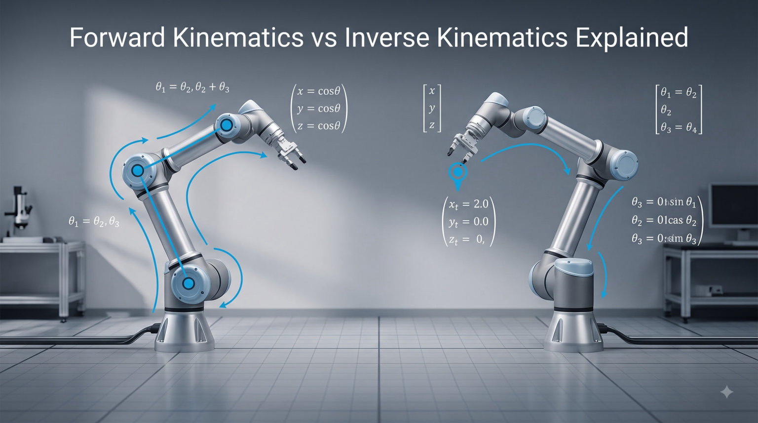
If you’ve ever tried to program a robot arm to pick up a cup, you’ve hit the same wall that catches most robotics builders: how do you tell a chain of joints exactly where to go? Forward Kinematics vs Inverse Kinematics is the core question that turns abstract joint angles into a working end effector, and turns a target position back into the angles that reach it. I’ve spent the last decade building and programming robotic arms, and these two concepts are the foundation of everything I do.

This guide walks you through both sides of that question, starting from the absolute basics and ending with a hands-on calculation you can reproduce on paper. Along the way you’ll get a comparison table that no other article on this topic offers, a step-by-step 2-DOF arm calculation you can verify with your own numbers, and a clear explanation of why Inverse Kinematics has a reputation as the hardest concept in robotics, and how to push past it. By the end, you’ll have the vocabulary, the math, and the practical context to pick the right method for your own project.

What Is Forward Kinematics?

Forward Kinematics is the process of calculating where a robot’s end effector will be when you set its joint angles. You feed in the joint values, and the math spits out the position and orientation of the tool at the end of the arm. It’s the simplest direction to compute because every input has exactly one output, and that output is deterministic.

Imagine a 3-joint robotic arm bolted to a table. If I tell joint 1 to rotate 30 degrees, joint 2 to rotate 45 degrees, and joint 3 to rotate 15 degrees, Forward Kinematics tells me exactly where the gripper sits in 3D space. No guessing, no iteration, no ambiguity.

The “kinematic chain” is the technical term for that series of connected links and joints. Each joint contributes a small transformation, and Forward Kinematics chains those transformations together from the base to the tip. The most common framework for doing this is the Denavit-Hartenberg convention, which assigns four parameters to each joint so the math stays consistent no matter how complex the arm gets. You’ll see DH parameters in every textbook and nearly every published FK derivation.

In animation and game development, Forward Kinematics is exactly what an animator does when they rotate the shoulder, then the elbow, then the wrist of a character rig. Every bone is rotated in sequence, and the hand lands wherever the chain of rotations puts it. That’s why character rigging tutorials always teach FK first, and why FK is the default animation mode in nearly every DCC tool.

The standard output of a Forward Kinematics calculation is a 4×4 homogeneous transformation matrix. The upper-left 3×3 block encodes the rotation of the end effector, and the rightmost column gives its position. Once you have that matrix, you can pull the position vector out, derive roll-pitch-yaw angles, or convert to a quaternion depending on what your downstream code needs.

What Is Inverse Kinematics?

Inverse Kinematics is the reverse problem: given where you want the end effector to be, calculate the joint angles that put it there. You give it a target position (and often an orientation), and the solver returns a set of joint angles that achieve it.

This sounds simple until you realize it’s not always solvable, and when it is, there may be multiple valid solutions. A 6-DOF arm with a target pose in its reachable workspace might have 8 different joint configurations that all put the gripper in the same place. The solver has to pick one, often optimizing for joint limits, energy use, or collision avoidance.

The IK problem is nonlinear, which is why beginners often hit a wall. Unlike FK, where you can write a single closed-form equation, IK usually requires either algebraic manipulation of trig equations, or numerical methods that iterate toward a solution. Both approaches have trade-offs, which we’ll cover later in this guide.

For a 2-DOF planar arm, you can solve IK on the back of a napkin with the law of cosines. For a 6-DOF industrial arm with arbitrary geometry, the closed-form solution might run to pages of algebra. Most real-world systems use numerical solvers: Jacobian pseudoinverse, Cyclic Coordinate Descent (CCD), or FABRIK.

In game engines like Unity and Unreal, IK is what makes a character plant its foot on a stair, or reach for a handhold on a wall. The animator sets the target, and the engine solves for the joint chain in real time. The same algorithms that bring characters to life are the ones running on factory robots.

Forward Kinematics vs Inverse Kinematics: Side-by-Side Comparison

This comparison table is the one I wish I had when I was learning. Most articles on Forward Kinematics vs Inverse Kinematics either bury the contrast in paragraphs or only cover one direction in detail. Here it is at a glance, and the table format is intentional: it gives you a single reference you can come back to without rereading the whole article.

Property	Forward Kinematics (FK)	Inverse Kinematics (IK)
Direction	Joint angles to end effector pose	End effector pose to joint angles
Input	Joint angles, link lengths	Desired position and orientation of end effector
Output	Position and orientation of end effector	Joint angles
Solution uniqueness	Always one solution	May have zero, one, or many solutions
Math complexity	Straightforward matrix multiplication	Nonlinear, often requires iteration
Solvability	Always solvable	Only if target is in reachable workspace
Computation cost	Low, deterministic	Higher, varies by method
Common methods	Denavit-Hartenberg transformation matrices	Analytical, Jacobian-based, FABRIK, CCD
Typical use cases	Animation rigs, trajectory playback, simulation	Pick-and-place, character foot planting, motion planning
Sensor requirement	Joint encoders only	Joint encoders plus target reference
Failure mode	None, output always valid	Singularities, unreachable targets, multiple solutions
Beginner friendliness	Easy to teach and visualize	Harder, requires comfort with trig or linear algebra
Real-time performance	Excellent	Depends on solver, can be slow on complex rigs
Joint limit handling	Set by the user directly	Must be enforced by the solver
Workspace awareness	Not required	Required to detect unreachable targets

The big takeaway: FK answers “where am I?” and IK answers “how do I get there?” Most real applications use both. You run FK to track where the arm actually is, then run IK to figure out what joint commands will move it to where you want next.

Key Concepts You Need to Understand First

Before you can pick a method or write code, you need five core ideas. I’ll define each in plain language, then show the math behind it. These are the terms you’ll see in every robotics paper, every product datasheet, and every forum thread about IK problems.

Degrees of Freedom (DOF)

Degrees of freedom are the number of independent ways a robot can move. A single revolute joint gives one DOF, meaning rotation about one axis. A 6-DOF arm like the ones used in manufacturing has six joints that together let it position and orient its end effector at any reachable pose in 3D space. More DOF gives more flexibility but makes IK dramatically harder, because more joints mean more unknowns to solve for.

End Effector

The end effector is the tool at the tip of the kinematic chain: a gripper, a welding torch, a paint sprayer, or even a character’s hand. Everything in FK and IK math is ultimately about controlling where this point ends up in space. In a robot arm, the end effector is usually defined relative to the last joint’s coordinate frame using a fixed transformation.

Kinematic Chain

A kinematic chain is the linked series of joints and rigid links connecting the base to the end effector. Open chains, like a robot arm, have a single path from base to tip. Closed chains, like a Stewart platform or a parallel mechanism, have loops. Closed chains make both FK and IK significantly more complex, which is why most educational material focuses on open chains.

Denavit-Hartenberg (DH) Parameters

DH parameters are a standardized way to describe each joint using four numbers: link length, link twist, joint offset, and joint angle. The DH convention makes it easy to write the homogeneous transformation matrix for each joint, then multiply them together to get the position of the end effector. Almost every FK derivation you’ll find online uses DH parameters, and once you understand them, you can describe any serial robot in a single table.

Jacobian Matrix

The Jacobian matrix relates joint velocities to end effector velocities. If you multiply the Jacobian by a vector of joint angle rates, you get the linear and angular velocity of the end effector. This is the foundation of most numerical IK solvers, which use the Jacobian inverse or pseudoinverse to iteratively step toward a target. The Jacobian also reveals singularities, configurations where the arm loses the ability to move in a particular direction.

Step-by-Step Example: Forward Kinematics for a 2-DOF Arm

Let’s work a real example. Consider a 2-DOF planar arm in the XY plane with two revolute joints. Joint 1 is at the origin, link 1 has length L1, joint 2 sits at the end of link 1, and link 2 has length L2 with the end effector at its tip.

I’ll use L1 = 5 units and L2 = 4 units, with theta1 = 30 degrees and theta2 = 45 degrees. Let me show you exactly how to find the end effector position. This is the same calculation my own team uses as a sanity check before testing more complex arms.

1. Write the position of joint 2 (end of link 1) using the first rotation: x1 = L1 cos(theta1), y1 = L1 sin(theta1). With our numbers: x1 = 5 × cos(30) = 5 × 0.866 = 4.330, y1 = 5 × sin(30) = 5 × 0.500 = 2.500.
2. Find the absolute angle of link 2 relative to the base: theta1 + theta2 = 30 + 45 = 75 degrees.
3. Compute the position of the end effector relative to the base by adding link 2’s contribution: x2 = x1 + L2 × cos(theta1 + theta2), y2 = y1 + L2 × sin(theta1 + theta2). That gives x2 = 4.330 + 4 × 0.259 = 5.366, and y2 = 2.500 + 4 × 0.966 = 6.364.
4. So the end effector is at approximately (5.366, 6.364) in the XY plane. That’s your FK result: given joint angles 30 and 45 degrees, the gripper lands at that point.

Now let’s check the inverse. If I wanted the gripper at (5.366, 6.364) with these link lengths, the IK equation comes from the law of cosines. The distance from the base to the target is r = sqrt(5.366² + 6.364²) = 8.317. Then theta2 = arccos((r² – L1² – L2²) / (2 × L1 × L2)) = arccos((69.17 – 25 – 16) / 40) = arccos(0.7043) ≈ 45.2 degrees, matching our input.

This same process scales to 6-DOF arms, but the math gets dense fast. That’s why most real-world IK solvers use matrices and iterative methods instead of trig by hand. If you want to verify this in code, the Python equivalent of step 3 is roughly: x2 = L1*math.cos(t1) + L2*math.cos(t1+t2), and the same for y2.

Quick Python Implementation

To make sure the math above is not just abstract, here is a short Python snippet you can copy and run. It implements both FK and IK for the 2-DOF arm we just worked through, and it should produce the same numbers I showed by hand. This is the same loop a real robot control system runs every few milliseconds, just with more joints and more decimals.

import math

# Forward Kinematics
def forward_kinematics(L1, L2, theta1_deg, theta2_deg):
    t1 = math.radians(theta1_deg)
    t2 = math.radians(theta2_deg)
    x = L1 * math.cos(t1) + L2 * math.cos(t1 + t2)
    y = L1 * math.sin(t1) + L2 * math.sin(t1 + t2)
    return (round(x, 3), round(y, 3))

# Inverse Kinematics (2-DOF, elbow-down solution)
def inverse_kinematics(L1, L2, x, y):
    r2 = x*x + y*y
    cos_t2 = (r2 - L1*L1 - L2*L2) / (2 * L1 * L2)
    cos_t2 = max(-1.0, min(1.0, cos_t2))
    theta2 = math.acos(cos_t2)
    theta1 = math.atan2(y, x) - math.atan2(L2 * math.sin(theta2), L1 + L2 * math.cos(theta2))
    return (round(math.degrees(theta1), 2), round(math.degrees(theta2), 2))

# Test it
print(forward_kinematics(5, 4, 30, 45))        # (5.366, 6.364)
print(inverse_kinematics(5, 4, 5.366, 6.364))  # (30.0, 45.2)

Run that snippet and you’ll see the FK call returns (5.366, 6.364) and the IK call recovers joint angles close to (30.0, 45.2). Once you have this working, you can extend it to 3-DOF, add orientation constraints, or swap the closed-form IK for a numerical solver.

Why Inverse Kinematics Is the Hardest Concept (and How to Push Past It)

If you ask robotics hobbyists what tripped them up the most, IK is almost always the answer. The reason isn’t that the math is impossible, but that beginners try to apply FK intuition to an FK problem. Three things in particular make IK feel like a wall, and once you see them, the wall gets shorter.

First, IK is nonlinear, so you can’t just invert a matrix. FK chains together linear rotations and translations, which makes its Jacobian straightforward to invert. IK inverts the whole chain, which mixes angles inside sine and cosine terms. That mixing is why there’s no closed-form “inverse FK matrix” the way there is for a 3D rotation. You have to use trig identities, geometric reasoning, or numerical iteration instead.

Second, IK has multiple valid answers and you have to pick one. FK is a function: one input, one output. IK is a relation: many inputs can produce the same output. For a 6-DOF arm aiming at a point in space, the solver might find four elbow-up configurations and four elbow-down ones, each a valid answer to the IK question. The solver needs extra rules (closest to current pose, minimum joint motion, away from joint limits) to choose one.

Third, IK can fail in ways that aren’t obvious. FK never fails: it always gives you a position. IK can return “no solution” because the target is out of workspace, or it can return a solution that drives the arm through a singularity. Beginners often treat IK as if it’s a function call that just works, and get confused when the arm jerks or stops moving. The fix is to test reachability before asking for a solution, and to clamp joint angles to physical limits inside the solver.

The way to push past these three issues is the same: keep the math small at first, work with a 2-DOF arm like the one above, and only add complexity after the simple case behaves. Then move to FABRIK or a Jacobian pseudoinverse, both of which handle a wide range of geometries without needing closed-form solutions. Once you see IK succeed on a 2-DOF arm and a 3-DOF arm, the 6-DOF case stops feeling like magic.

When to Use Forward Kinematics vs Inverse Kinematics

The choice depends on what you already know and what you’re trying to control. Here’s how I decide in my own projects, and these rules transfer to almost any robot or rig you’ll build.

• Use Forward Kinematics when you want to control each joint independently, animate a character by rotating bones in sequence, simulate a known trajectory, or verify that a set of joint commands produces the pose you expect.
• Use Inverse Kinematics when you have a target position and orientation for the end effector and need the joint angles to reach it. This covers pick-and-place, foot planting on uneven terrain, and any application where you think in terms of “where” rather than “how.”
• Use both when you’re building a full motion pipeline. Plan a path in task space using IK, then check the resulting joint motion with FK, then drive the actual motors using the joint angles from the IK output.
• Prefer analytical IK when your robot has a spherical wrist or simple geometry. Closed-form solutions are fast and exact, with no iteration required.
• Prefer numerical IK when the geometry is irregular or you want a general-purpose solver that works across robot types. Jacobian-based solvers and FABRIK handle a wide range of configurations but iterate per frame.

For most robotics hobbyists, the rule of thumb is: build and test in FK, then add IK once you need target-driven motion. Trying to start with IK on day one is the most common reason beginners give up.

Real-World Applications of FK and IK

Forward and Inverse Kinematics show up wherever there’s a kinematic chain. Here are the fields I see them used most, and the specific roles each plays.

Industrial robotics: A 6-axis arm on a manufacturing line uses IK to plan a path from a bin to a conveyor, then FK to verify the trajectory before execution. Welding robots, paint sprayers, and CNC mill tool changers all rely on this pair. The whole class of “programming by demonstration” tools work by recording joint angles (FK) and then replaying them at higher speed.

Medical robotics: Surgical robots like the da Vinci system use IK to translate a surgeon’s hand motion into precise instrument tip motion. The slave arms solve IK at hundreds of hertz to keep the tip exactly where the master controller commands. Haptic feedback loops depend on FK to report the actual position of the instruments back to the surgeon’s controls.

Animation and game development: Riggers use FK for the body of a character animation, then IK for foot locking, hand planting, and procedural adjustments. Modern engines like Unity and Unreal expose IK solvers that take a target transform and produce joint rotations in real time. Look at any AAA game and you’ll see IK handling the player’s foot placement on stairs and ladders.

Virtual reality: Full-body VR tracking often uses IK to estimate the pose of a user’s hidden limbs from a small number of tracked points. Head, hands, and feet trackers are run through an IK solver to recover the joint angles of elbows, knees, and spine. This is why a VR avatar can move convincingly with only three sensors.

Motion platforms and simulators: Stewart platforms use IK to convert a desired cockpit pose into six actuator lengths. FK confirms that the resulting actuator lengths correspond to the desired motion. Flight simulators and driving simulators depend on this pair running at frame rate.

CNC machining and 3D printing: Tool paths are planned in Cartesian space, then IK (or its cousin, inverse dynamics) converts them into motor commands for each axis. FK verifies the commanded motion before the cut starts.

Advanced Topics: Singularities, Workspace, and IK Methods

Once you start solving real IK problems, three concepts come up constantly. You don’t need to master them on day one, but you should know they exist before you debug a stubborn robot.

Singularities are joint configurations where the Jacobian loses rank. Near a singularity, the arm cannot move in one or more directions, and small joint motions produce huge end effector velocities. The classic example is a 6-DOF arm fully stretched out: it can swing its end effector in a circle but cannot push it further out. Most IK solvers detect singularities and damp the joint velocities to avoid runaway commands.

Workspace is the set of all positions the end effector can reach. The reachable workspace is bounded by link lengths; the dexterous workspace is the subset where the arm can reach with full orientation. Targets outside the workspace have no IK solution, and well-designed solvers return a clear failure instead of producing nonsense angles.

IK solving methods split into two camps. Analytical methods like the Paden-Kahan subproblems produce exact closed-form solutions but only work for specific robot geometries. Numerical methods like the Jacobian pseudoinverse, Cyclic Coordinate Descent (CCD), and FABRIK iterate toward a solution and work on any kinematic chain. Trade accuracy and joint-limit handling for generality and computational cost.

Frequently Asked Questions

Conclusion

Forward Kinematics and Inverse Kinematics are two sides of the same coin: one tells you where you are, the other tells you how to get where you want. Once you’ve worked a 2-DOF arm by hand and built a comparison table in your head, the rest of the field starts to click into place. The math gets heavier as DOF grows, but the core idea stays simple, and the same comparison table in this article will keep scaling with you.

My recommendation for builders reading this in 2026: start with FK on a 2-DOF arm, then add a Jacobian-based IK solver, then push toward a 6-DOF platform with both FK and IK running in your control loop. That progression covers the same ground most robotics engineers walk over their first year, and you’ll come out the other side with a real working system. Bring the comparison table to your bench, work the 2-DOF example with your own link lengths, and you’ll have the foundation to tackle any kinematic chain that comes next.