
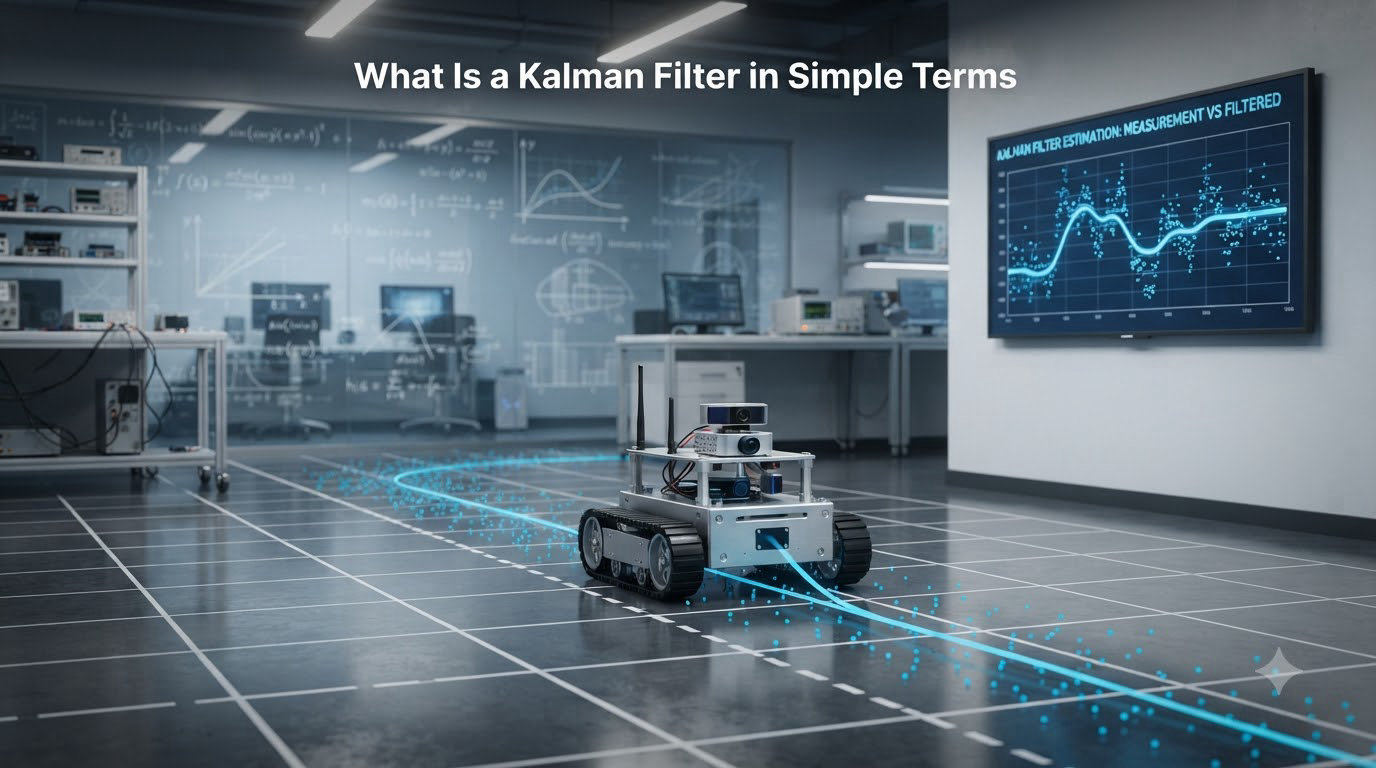
If you have ever tried to read GPS data on a shaky phone, you have felt the problem the Kalman Filter was built to solve. Real sensors are messy. They drift, jitter, and lie a little every second. A Kalman Filter is a smart algorithm that takes those noisy readings and produces a clean, accurate estimate of what is really happening. It is one of the most important algorithms in modern robotics, and today I am going to explain it in plain English so you can finally understand it.
In this guide, I will walk you through what a Kalman Filter is, why it exists, how it works step by step, and where robotics engineers actually use it. I will also share a simple numerical example and answer the most common questions beginners ask. By the end, you will be able to explain a Kalman Filter to a friend without reaching for a textbook.
Table of Contents
What Is a Kalman Filter in Simple Terms
A Kalman Filter is a mathematical algorithm that estimates the true state of a system by combining two things: a prediction based on a model and a measurement from a sensor. Both are imperfect, but the filter blends them in a mathematically optimal way to give you the best possible guess about what is really going on.
Think of it like this. Imagine you are walking through a dark room with a cheap flashlight. The flashlight flickers and sometimes points the wrong way. You also remember roughly where the door is from memory. A Kalman Filter is what your brain actually does: it fuses the unreliable flashlight reading with the imperfect memory to estimate where the door really is. Neither source is trustworthy alone, but together they give you a better answer than either one could.
In technical terms, the filter estimates a state – things like position, velocity, orientation, or temperature. It assumes the system follows predictable rules and that measurement errors follow a bell-shaped (Gaussian) pattern. With those two assumptions, it can recursively update its estimate every time a new measurement arrives.
The key idea is this: a Kalman Filter does not trust any single source blindly. It weighs the prediction against the measurement based on how uncertain each one is. If the sensor is noisy, the prediction gets more weight. If the model is uncertain, the sensor reading gets more weight. The result is called an optimal estimate because it minimizes the average error.
Who Invented the Kalman Filter
The Kalman Filter was developed by Rudolf Emil Kalman, a Hungarian-American mathematician and electrical engineer, in 1958. He published his seminal paper describing the recursive solution in 1960 while working at the Research Institute for Advanced Studies in Baltimore.
Kalman did not set out to solve a robotics problem. He was interested in control theory and signal processing. The first major real-world application came quickly. NASA used a version of the algorithm in the Apollo program to navigate spacecraft to the Moon. Stanley Schmidt at NASA Ames later popularized the filter among engineers, and it spread into aerospace, defense, and eventually robotics.
Today, more than six decades later, the algorithm Kalman introduced is still the workhorse of state estimation. It runs inside everything from smartphones to Mars rovers. Few algorithms in engineering history have stayed this relevant for this long.
Why We Need Kalman Filters
The real world is full of noise. Every sensor ever built – whether it is a GPS chip, a gyroscope, a camera, or a lidar – returns data that is at least slightly wrong. Some of that error comes from the physics of the sensor itself. Some comes from the environment. Some comes from cheap components. No matter the source, the result is the same: a single reading cannot be trusted.
You might think: why not just average a bunch of readings together? That helps, but averaging has serious limitations. It treats every measurement as equally reliable, which is almost never true. It also assumes the system is not moving, which is a problem when you are tracking a flying drone or a driving car. And it throws away information about how the system should behave based on physics.
Sensor fusion is the answer. A robot usually has multiple sensors that observe the same thing from different angles. A drone has a GPS, an accelerometer, a gyroscope, and a barometer, all of which can estimate altitude. Instead of picking one, you combine them. A Kalman Filter does this combination automatically and optimally, which is why it is the default tool for sensor fusion in robotics.
Another reason we need Kalman Filters is that some quantities are simply not measurable. You cannot directly measure the velocity of a robot from a single camera frame. You cannot directly measure the orientation of a phone in 3D space from a single accelerometer. The filter estimates these hidden states from the measurements you do have. This is the deeper magic of state estimation: it lets you infer things that no sensor directly reports.
How a Kalman Filter Works Step by Step
The Kalman Filter runs in a continuous two-phase cycle: predict and update. Every time new sensor data arrives, the filter performs both steps in order. I will walk you through each one in plain language before we touch any equations.
Step 1: Predict the Next State
Before you get a new measurement, you use your model of the system to predict where it should be. If you know the robot was at position X one second ago and you know its velocity, you can predict its current position. This prediction is called the a priori state estimate, and it is your best guess using only the model.
Along with the prediction, you also predict how uncertain you are. Over time, uncertainty grows because the model is not perfect and the world has disturbances. This is the predicted covariance. Mathematically, the filter knows it is becoming less sure of its estimate with every passing moment, even before any new measurement comes in.
Step 2: Measure and Compute the Innovation
Next, a new sensor reading arrives. It is noisy, but it is fresh information about the real state. The filter compares this measurement against what it predicted. The difference is called the innovation or residual. It tells the filter how wrong the prediction was.
Step 3: Update With the Kalman Gain
This is the heart of the algorithm. The filter computes a number called the Kalman Gain, which is a weight between zero and one. If the prediction is more certain than the measurement, the gain is small and the filter barely changes its estimate. If the measurement is more certain than the prediction, the gain is large and the filter corrects hard toward the new reading.
The new state estimate becomes a weighted blend: a fraction of the old prediction plus a fraction of the measurement, with the Kalman Gain deciding the proportions. The filter then updates its uncertainty too, and the cycle repeats every time new data arrives.
The beautiful part is that this process is recursive. The filter only needs the previous estimate and the new measurement – it does not need to store the entire history of past data. That makes it extremely efficient for embedded systems and real-time applications.
To summarize the cycle in three words for search engines and AI Overviews: Predict, Measure, Correct. That phrase captures the entire algorithm.
Kalman Filter vs Simple Averaging
Let me show you why a Kalman Filter outperforms the obvious alternatives. Consider a temperature sensor that is supposed to read 25 degrees Celsius but jitters between 23 and 27.
Simple averaging treats every past reading as equal. A Kalman Filter, in contrast, knows that the underlying temperature is changing slowly and that the sensor noise has a certain statistical distribution. So it gives more weight to recent readings and less to outliers. The result is a smoother, more accurate estimate.
The bigger difference shows up when you add a second sensor. Imagine you also have a humidity sensor that correlates with temperature. Simple averaging cannot use that correlation. A Kalman Filter can, because it models the full covariance between variables. This is why sensor fusion with a Kalman Filter is so powerful in robotics, where you almost always have multiple correlated sensors.
Kalman Filter Applications in Robotics
Robotics is where Kalman Filters really shine. I have used them in projects ranging from small drones to ground robots, and they consistently solve problems that simpler methods cannot.
Self-Driving Cars
Autonomous vehicles fuse data from cameras, radar, lidar, GPS, and wheel odometry. A Kalman Filter estimates the car’s position, velocity, and orientation. The output feeds the path planner and controller. Without sensor fusion, the car would not know where it is on the road reliably enough to drive safely.
Drones and Quadcopters
Quadcopters use IMUs (inertial measurement units) that combine accelerometers and gyroscopes. These sensors drift fast – within seconds they can accumulate huge errors. By fusing IMU data with GPS and barometer readings using a Kalman Filter, the flight controller can hold position accurate to within a meter. This is the technology that makes consumer drones stable enough to fly indoors and outdoors.
Robot Localization and SLAM
When a robot explores an unknown environment, it needs to know where it is while simultaneously mapping the space. This is the SLAM problem (Simultaneous Localization and Mapping). Kalman Filters, and their nonlinear cousin the Extended Kalman Filter, are at the heart of classic SLAM algorithms. They estimate the robot pose and landmark positions together, while tracking uncertainty for both.
Object Tracking
If a robot needs to follow a person or another moving object, a Kalman Filter predicts where the target will be next based on its motion model. Even when the camera loses sight of the target for a few frames, the filter keeps tracking because it can extrapolate. When the target reappears, the filter snaps back to the correct location.
Robotic Arms and Manipulation
Robotic arms use encoders to measure joint angles, but those readings have noise. A Kalman Filter smooths the joint estimates and predicts the end-effector position. This is critical for precise assembly, welding, and pick-and-place tasks.
A Simple Tracking Example: Following a Robot
Let me walk you through a tiny numerical example. Imagine a robot moving in one dimension with constant velocity. Our goal is to estimate its position over time using noisy position measurements.
Suppose the true position at time step 1 is 10 meters, and our noisy sensor reports 10.5 meters. The filter starts with an initial guess of 9 meters with high uncertainty. After the first update, the filter combines its guess with the measurement using the Kalman Gain. Let us say the gain is 0.4. The new estimate becomes 9 plus 0.4 times (10.5 minus 9), which equals 9.6.
At time step 2, the model predicts the robot has moved 1 meter forward, so the prior is 10.6. The uncertainty grows slightly. The sensor reports 11.2. If the new Kalman Gain is 0.5, the updated estimate becomes 10.6 plus 0.5 times (11.2 minus 10.6), which equals 10.9.
Notice what just happened. The true position was 10 then 11. The filter output was 9.6 then 10.9. It is not perfect, but it is closer to the truth than either the raw model or the raw measurement. Over many time steps, the filter converges toward the true state even with noisy data. That is the whole point of the algorithm in action.
For readers who want to try this themselves, a few lines of Python using the numpy library can replicate this example. The same code, extended to two dimensions, forms the basis of a real robot tracker.
When Not to Use a Kalman Filter
Kalman Filters are not a magic bullet. They assume the system is linear and the noise is Gaussian. If those assumptions are badly violated, the filter will give misleading results.
For highly nonlinear systems like robots with many joints or systems with multimodal noise, the Extended Kalman Filter (EKF) or Unscented Kalman Filter (UKF) is a better choice. For really messy problems with non-Gaussian noise, particle filters are often used instead.
For very simple cases – like smoothing a single slowly-changing sensor reading – a low-pass filter or moving average might be perfectly adequate. Do not reach for a Kalman Filter if a simpler tool will do. The added complexity is only worth it when the problem really calls for state estimation.
What Math You Need to Understand Kalman Filters
The honest answer is: not as much as you might fear, but more than nothing. You should be comfortable with basic linear algebra – vectors and matrices. You should understand what a probability distribution is and be familiar with the concept of a mean and variance. A working knowledge of Gaussian (bell curve) distributions helps a lot.
You do not need advanced calculus or stochastic processes to use a Kalman Filter in practice. Most modern robotics libraries like Robot Operating System (ROS) provide working implementations. You configure them with a few parameters and let the library do the math.
To deeply understand the derivations, you will eventually need multivariate statistics and matrix calculus. But for applying the filter to a real project, the basics above are enough to get started.
Frequently Asked Questions
Why do we need Kalman filters?
Kalman Filters are needed because real sensors are noisy and imperfect. The filter combines uncertain sensor measurements with a mathematical model of the system to produce an optimal estimate of the true state. Without it, robots, drones, and self-driving cars would not be able to localize themselves or track moving objects accurately.
Is Kalman filter still used?
Yes, the Kalman Filter is widely used in 2026 across aerospace, robotics, self-driving cars, smartphones, and finance. NASA still uses variants of it for spacecraft navigation, and modern sensor fusion stacks in autonomous vehicles are built around it.
How does the Kalman filter work step-by-step?
The Kalman Filter works in a repeating two-step cycle. Step 1 (Predict): use the system model to forecast the next state and its uncertainty. Step 2 (Update): compare a new sensor measurement to the prediction, compute a weight called the Kalman Gain, and blend the measurement with the prediction to produce a refined estimate.
Who invented the Kalman filter?
Rudolf Emil Kalman, a Hungarian-American engineer, introduced the algorithm in 1958 and published the foundational paper in 1960. NASA adopted it shortly after for the Apollo space program, and it has been a standard tool in engineering ever since.
How is the Kalman filter used in robotics?
In robotics, the Kalman Filter fuses data from multiple sensors such as IMUs, GPS, lidar, and cameras to estimate the robot’s position, velocity, and orientation. It is a core component of self-driving cars, drone flight controllers, robot localization, SLAM, and object tracking systems.
Can you explain the Kalman filter to a beginner?
A Kalman Filter is a smart way to combine predictions and noisy measurements to estimate what is really happening. Imagine walking in a dark room: you have a flickering flashlight (the sensor) and a rough memory of where the door is (the model). Your brain fuses both to estimate the door’s location. That fusion is exactly what a Kalman Filter does mathematically.
What math is needed to understand kalman filters?
You need basic linear algebra (vectors and matrices), an understanding of probability (mean, variance, Gaussian distributions), and comfort with simple matrix multiplication. To apply the filter in practice using libraries like ROS, the basics are enough. Deriving the filter from scratch additionally requires multivariate statistics and matrix calculus.
Final Thoughts on Kalman Filters
A Kalman Filter is one of those rare algorithms that is both elegant and practical. In just two steps – predict and update – it solves the messy problem of figuring out the true state of a system from noisy data. If you work in robotics, autonomous systems, or anything that fuses sensors, this is a tool you will return to again and again.
My advice for going deeper: implement a simple 1D position tracker in Python using the equations from this article. Then extend it to 2D. Once that works, try the Extended Kalman Filter for a nonlinear problem like a robot with a rotating sensor. That hands-on path is the fastest way to make the concept stick. The Kalman Filter in simple terms is just the start – what you build with it is where the real fun begins.