What Is Robot Path Planning (September 2026 Complete Guide)

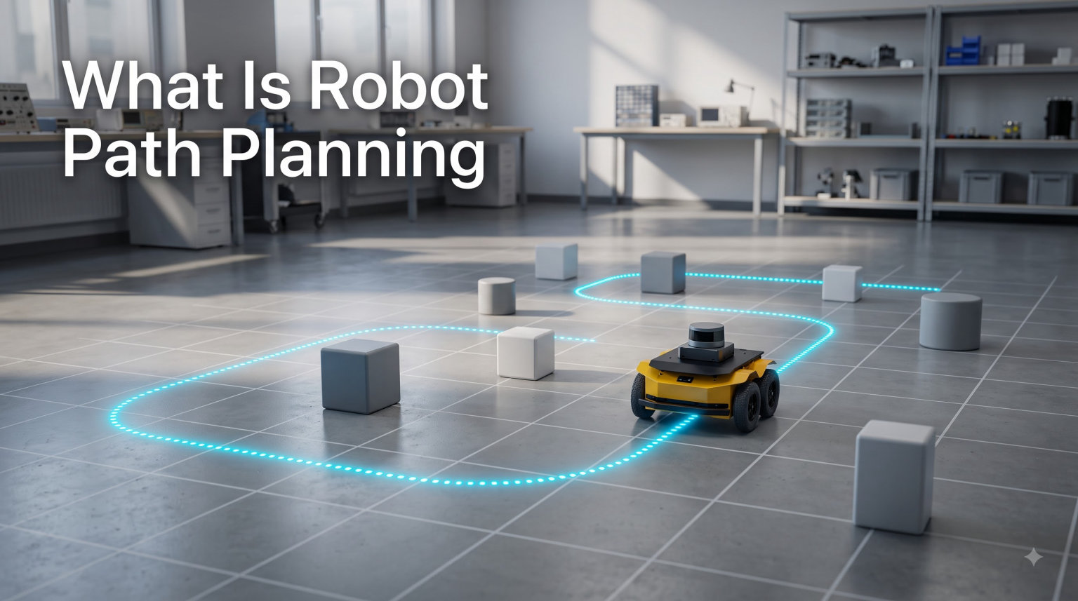
Robot path planning is the computational process of finding a safe, collision-free route from a robot’s starting point to a target destination while avoiding obstacles. I first ran into the term while building a small indoor rover a few years ago, and it took me weeks to realize that “path planning” was a distinct field with its own algorithms, math, and decades of academic history.

If you have ever asked yourself “how does a robot actually decide where to go?”, this guide is for you. I will walk you through the full picture: what robot path planning means, how it works under the hood, the algorithms behind it, and where you see it used in the real world. By the end, you will understand the difference between path planning, motion planning, and trajectory planning, and you will know which algorithm fits which problem.

Let us start with the clearest possible definition.

Robot Path Planning Definition: What It Means and Why It Matters

Robot path planning is the process of computing a sequence of waypoints or configurations that move a robot from a start state to a goal state without colliding with obstacles. The “path” can be a curve in 2D space, a route through a 3D warehouse, or a trajectory through a many-dimensional configuration space that describes every joint of a robotic arm.

You will see the same idea described in three slightly different ways across textbooks and papers:

• Path planning focuses on the geometric route.
• Motion planning adds the robot’s physical constraints, like steering limits and joint ranges.
• Trajectory planning adds time and velocity, producing a schedule of positions rather than just a shape.

All three share the same goal: get the robot from A to B without hitting anything. The difference is how much of the robot’s physical reality the algorithm has to respect.

Why does it matter? Because the moment a robot is asked to operate without a human holding the joystick, it must answer the question “where do I go next?” by itself. That single question drives warehouse logistics, autonomous vehicles, surgical robots, and the Mars rovers you read about in the news. I covered related industry news in the Path Robotics deal coverage at Smashing Robotics, and path planning sits right at the heart of every company mentioned.

How Robot Path Planning Works: The Step-by-Step Process

Path planning works by representing the environment as a searchable map, then using an algorithm to find an optimal route from start to goal. Every planner, no matter how fancy, runs through roughly the same four steps.

1. Sense or build the environment. The robot uses sensors such as cameras, LiDAR, or a pre-loaded floor plan to build a map of where it is and what is around it.
2. Represent the world as data. The map is converted into a form the algorithm can search: a grid, a graph, a tree, or a continuous function.
3. Search for a feasible path. The algorithm explores the representation and returns a sequence of moves that avoids obstacles and respects constraints.
4. Execute and re-plan if needed. The robot follows the path. If something new appears, the planner re-runs in real time to find a safer route.

That last step is where modern systems shine. Self-driving cars, for example, do not just plan once and drive. They re-plan every few hundred milliseconds because the world keeps changing.

Map Representation and Environment Modeling

Before any algorithm can run, the environment has to be turned into numbers. The most common representations are:

• Occupancy grids – the world is sliced into small squares or cubes, and each cell is marked free, occupied, or unknown. A* and Dijkstra both work beautifully on grids.
• Roadmaps – a graph of “milestone” points connected by safe edges, like a sparse skeleton of free space.
• Geometric primitives – obstacles described as polygons or spheres, useful for robot arms in structured workspaces.
• Point clouds – raw 3D scans from depth cameras, which sampling-based planners like RRT can use directly.

For mobile robots in warehouses, occupancy grids are by far the most common. For robot arms, geometric primitives are typical because the workspace is small and the geometry is well known.

Configuration Space (C-Space) Explained

The configuration space, often shortened to C-space, is the mathematical playground where path planning actually happens. Instead of thinking about the robot as a rigid shape in 2D or 3D, you describe the robot by a single point in a higher-dimensional space where each axis represents one degree of freedom.

Imagine a simple robot arm with two joints. In the real world, it sweeps through 2D space. In C-space, the arm is a single dot whose coordinates are (joint 1 angle, joint 2 angle). A 6-DOF industrial arm becomes a point in 6-dimensional space. Self-driving cars are usually modeled in a 2D or 3D C-space (x, y, heading).

The genius of this idea is that collision checking becomes a simple point-in-region test. You mark which configurations of the robot would cause a collision as “C-space obstacles,” and the planner just has to find a curve through the free region. This is the foundation laid out in the classic Wikipedia motion planning article, and it is still the standard mental model used in robotics textbooks.

Global vs Local Path Planning: Key Differences Explained

Global path planning computes a full route from start to goal using a known or pre-built map, while local path planning reacts in real time to whatever the robot’s sensors see right now. Most real robots use both at the same time.

Here is a quick mental model I use with my students:

• Global planner is the GPS navigator. It knows the whole city and can pick the best highway route, but it does not know about the accident up ahead.
• Local planner is the driver. It only sees 20 meters of road, but it can swerve to miss a pothole.

Self-driving cars run a global planner over the road network and a local planner over the live sensor data, then merge the two. A typical setup might use A* for the global layer and Dynamic Window Approach (DWA) or a potential field for the local layer. The same pattern shows up in mobile robots, drones, and even vacuum cleaners.

Global planners tend to be more thorough but slower. Local planners are fast and reactive but can get stuck if there is no good global hint guiding them. Pairing the two is what gives you the best of both worlds.

Path Planning vs Motion Planning: What’s the Difference?

Path planning produces a geometric route, while motion planning adds the robot’s physical constraints to produce a route the robot can actually drive or move along. In practice, you will often see the terms used interchangeably, but they are not the same thing.

A path is a curve in space. A motion is a path plus the timing, velocities, and accelerations needed to follow it. A motion planner also enforces things like:

• Maximum wheel speed for a mobile robot
• Joint limits and torque limits for a robot arm
• Non-holonomic constraints, meaning the robot cannot slide sideways like a car
• Dynamic obstacles that move over time

For beginners, the safe rule is: if you only care about the shape of the route, you are doing path planning. If you also care about whether the robot can physically execute it, you are doing motion planning. Trajectory planning sits one level above that and bakes in time as well.

Main Path Planning Algorithms Compared

There are four path planning algorithms you will see again and again in robotics: A*, Dijkstra, RRT, and Potential Fields. Each one solves a different kind of problem, and the right choice depends on your map type, dimensionality, and whether you need an optimal answer or just a fast one.

Algorithm	Best For	Optimal?	Strengths	Weaknesses
A*	Grid maps, mobile robots	Yes (with admissible heuristic)	Fast, easy to tune, finds shortest path	Struggles in high dimensions
Dijkstra	Small grids, guaranteed optimality	Yes	No heuristic needed, simple to implement	Slow on large maps
RRT / RRT*	High-dimensional spaces, robot arms	RRT: no. RRT*: asymptotically yes	Scales to many dimensions, handles complex geometry	Paths are jagged, need post-smoothing
Potential Fields	Real-time local planning, simple robots	No	Very fast, simple math, smooth motion	Can get stuck in local minima

Below is a closer look at each one.

A* Algorithm

A* (pronounced “A-star”) is the workhorse of grid-based path planning. It is a graph search that combines the actual cost from the start with a heuristic estimate of the cost to the goal, and it expands the most promising nodes first. With a good heuristic, A* returns the shortest path and does so much faster than Dijkstra because it ignores dead ends.

I default to A* whenever I am working on a 2D map with cells no smaller than a few centimeters. It is the algorithm behind most indoor mobile robot navigation stacks, and it is the same one you would use to find a path through a video game maze.

Dijkstra’s Algorithm

Dijkstra’s algorithm is the grandparent of A*. It expands nodes in order of distance from the start until it reaches the goal, and it is guaranteed to find the optimal path. The downside is that it explores in every direction, so on a large map it wastes time on regions that are clearly not useful. A* fixes that by adding a heuristic to point the search toward the goal.

In modern robotics, Dijkstra is mostly used as a reference or as a teaching tool. If your map is small or you genuinely need the cheapest path with no shortcuts, Dijkstra is a safe pick.

RRT and RRT*

Rapidly-exploring Random Trees (RRT) are sampling-based planners that shine in high-dimensional configuration spaces. The algorithm grows a tree of valid configurations by sampling random points and connecting them to the nearest existing node, which avoids having to build a full grid of every possible state. RRT* improves on RRT by rewiring the tree to converge toward an optimal solution as you give it more time.

For 6- or 7-DOF robot arms, or any robot with many degrees of freedom, RRT and RRT* are usually the right call. They are slower per query than A* but they scale to problems where a grid would be impossible. The output is often jagged, so production systems typically run a path smoother over the result.

Potential Fields Method

Potential fields treat the robot like a positively charged particle, the goal like a negatively charged attractor, and obstacles like positively charged repellers. The robot “rolls downhill” through the combined field until it reaches the goal. It is computationally cheap and produces smooth motion, but the algorithm can get trapped in local minima where the attractive and repulsive forces cancel out.

You will see potential fields used as a local planner paired with a global planner. Modern variants add random walks or virtual goal points to escape those dead spots, and the basic idea still shows up in reactive obstacle avoidance for drones and robot arms. The MIT path planning lecture notes include a solid walkthrough if you want the original derivation.

Real-World Applications of Robot Path Planning

Path planning is the invisible engine behind most of the robotics news you read. A few examples I have followed closely:

• Self-driving cars. Companies like Waymo, Cruise, and Tesla use a layered planner: a global route over the road network and a local planner over real-time sensor data.
• Warehouse robots. Amazon, Symbotic, and others run thousands of mobile robots in the same building, all planning around each other in real time. Safety scaling is a huge topic – I covered it in the warehouse robot fleet safety webinar.
• Robot arms in manufacturing. 6-DOF arms use RRT variants to plan around fixtures and parts.
• Aerial drones. UAVs running visual SLAM use local planners to dodge branches, walls, and other drones.
• Surgical robots. Da Vinci-style systems use motion planning to keep tools outside patient anatomy while still reaching the surgical site.

Anywhere a robot has to move through space without a human driving it, path planning is part of the stack. It is the layer that turns raw sensing into a deliberate route.

Common Challenges in Path Planning

Once you move past toy examples, path planning gets hard quickly. The most common pain points I have seen in the r/robotics community and in my own projects are:

• High-dimensional spaces. Grid methods blow up exponentially with degrees of freedom. A 6-DOF arm has a grid with millions of cells per axis, which is why sampling planners exist.
• Dynamic obstacles. People, pets, and other robots move. A precomputed path becomes unsafe the moment a new obstacle shows up, so re-planning has to be fast.
• Uncertainty in sensing. LiDAR and cameras are noisy. Planners have to either clean the map first or reason about uncertainty directly.
• Local minima. Potential fields and similar reactive methods can get stuck in places where the forces balance out.
• Real-time performance. Most mobile robots need to re-plan in under 100 ms, which rules out slower optimal algorithms on large maps.

These are the same problems that drive current research, including the integration of learned models that predict where obstacles will move next.

Frequently Asked Questions

Final Thoughts on Robot Path Planning

Robot path planning is what turns a sensor-equipped machine into something that can move on its own. Start with a clear map, pick an algorithm that matches your dimensionality and timing budget, and pair a global planner with a reactive local one if the world is dynamic. Once you have a working pipeline, you can layer in trajectory optimization and learned models to push performance further.

If you are building something hands-on, the fastest way to learn is to drop A* into a 2D grid simulator, watch it solve a maze, then swap in RRT and see how the behavior changes in higher dimensions. If you want to keep going, the robot chassis guide and the planetary gearbox article are good places to see how the rest of the robot supports the planner. Also check out the backlash in robot gearing piece – that mechanical tolerance directly affects how cleanly your motion planner can execute its paths.